This is Part 1 of a three part series.  The efficient market hypothesis in financial economics holds that prices reflect all available information.  An implication of the theory is that it is impossible to beat the market on a risk-adjusted basis.  If the theory holds, the best investment strategy would be to buy a low cost index fund that mirrors the holdings of the market.  Active security selection takes a view that it is possible to find undervalued securities.

A factor is simply some attribute of a group of securities that help explain the returns.

If we can define a factor that explains asset returns, we could simply buy more of those assets or stocks and generate a higher return or a similar return at a lower risk.  Factor investing is also marketed as ‘strategic beta’, ‘smart beta’ or ‘semi-passive investing’.   Generally, funds that employ factor-based investing have an expense ratio that is lower than funds with active security selection, but slightly higher than funds which follow the core stock market index.  In recent years, inflows into Exchange Traded Funds (ETFs) have eclipsed mutual fund inflows.  Low cost index funds dominate the asset base.  According to Morningstar Research ‘A Global Guide to Strategic Beta Exchange Traded Products’, published in September 2016, there are over 1123 US exchange trade products in the strategic beta category.  The combined assets are worth over $550 billion dollars.  Assets grew 17% over the prior year.

Fama and French 3-Factor Model

To help explain factors let’s get into the details of the value factor and the small cap factor.  You may have heard expressions such as ‘value stocks outperform the stock market’ or ‘I am a value investor’ or ‘small cap stocks beat large cap stocks’.  These factors were introduced in the now famous Fama and French 3-Factor Model in 1992.   Eugene Fama and Kenneth French were professors at the University of Chicago Booth School of Business.

The Fama and French 3-Factor Model showed that stock performance can be explained by additional factors besides the overall market risk.  More specifically, it says that stock return can be explained by the overall return of the market, along with a value factor and a small market capitalization factor.

What is the Value Factor and the Small Cap Factor?

Fama and French defined a variable (or factor) we know as the value factor, HML.  HML stands for ‘high minus low’ and refers to the book value of the company divided by the market value of a company.  The book value of a company is what the company would be worth if we sold it off.  It is the value of the assets minus liabilities and intangibles such as patents or acquisition goodwill.  The market value of the company is the total shares outstanding times the current price of the stock.  To derive the HML factor, Fama and French grouped companies into quintiles based on the value of their book value to market value.  The HML factor is the mean return difference between those companies in the highest book to market minus the lowest book to market values

For the small market cap factor, Fama and French defined the SMB factor (small minus big).  SMB is the return generated in a similar fashion to HML.  The return for the stocks with the smallest market capitalization is subtracted from the stocks with the largest market capitalization.

What Evidence Do We Have?  A Regression Detour

To understand the significance of these factors it helps to understand the basics of linear regression and statistics.

Linear regression is the process of taking a sample of data and fitting the best straight line that explains the data.  For example, consider the monthly returns for Verizon compared with the monthly market return premium over risk free bonds.  In the following figure I have plotted the monthly market return premium from the Fama and French data set on the x axis.  On the y axis, I have Verizon monthly returns from Dec 1983 through Feb 2017 (the last month for which Fama and French have updated their data).

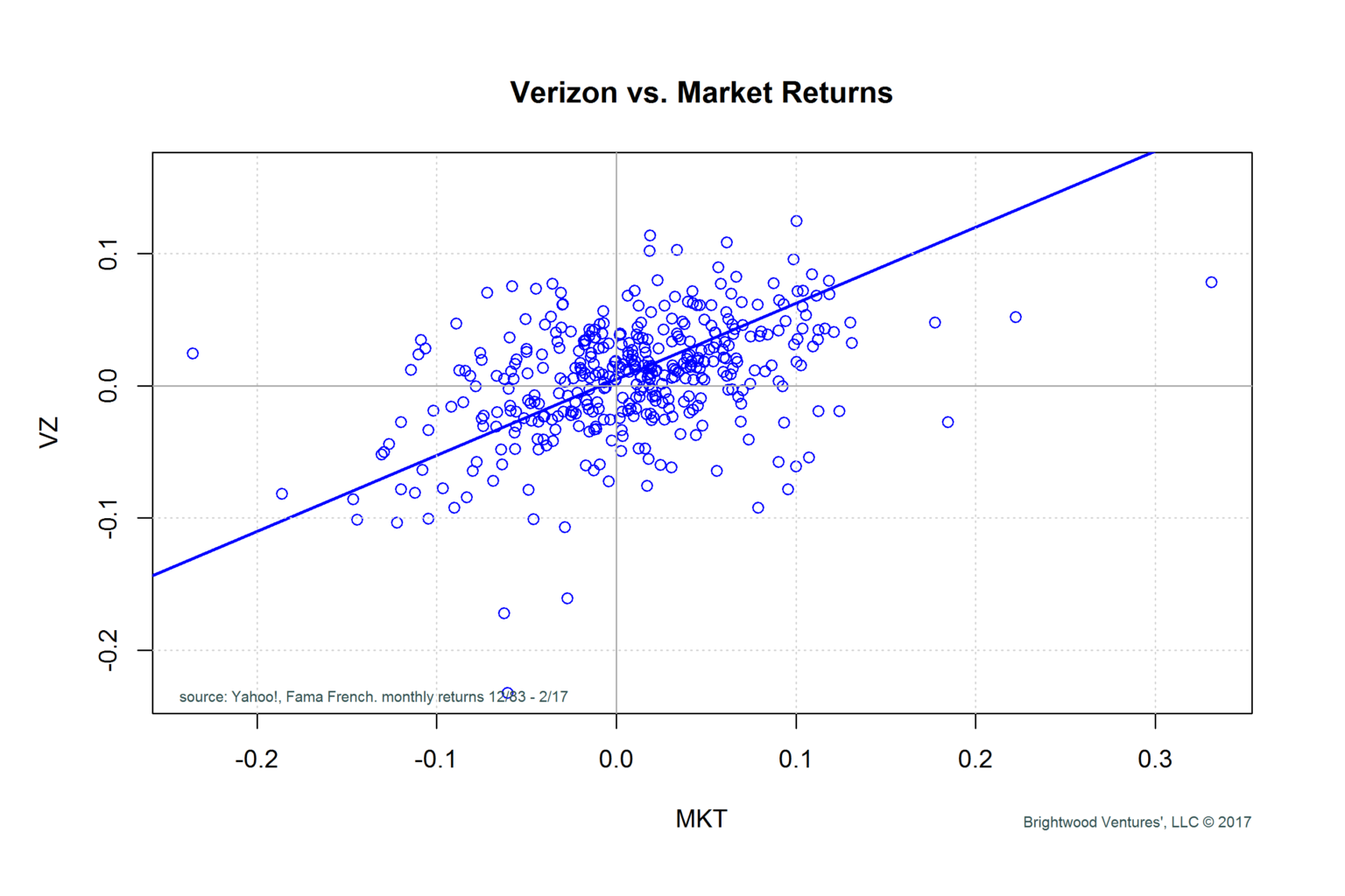
Linear regression is the mathematical process of fitting a line to a set of points. The line that minimizes the error between the points and the line is the best fit.

We can express the relationships as: VZ = alpha + Beta (Market Premium).

Using R programming, I ran regression for this data. The results are as follows:

Call:
 lm(formula = VZ ~ MKT)

Residuals:
 Min 1Q Median 3Q Max
 -0.254523 -0.035314 0.001834 0.032966 0.281239

Coefficients:
 Estimate Std. Error t value Pr(>|t|)
 (Intercept) 0.004840 0.002871 1.686 0.0927 .
 MKT 0.575548 0.064550 8.916  ---
 Signif. codes: 0 ‘***’ 0.001 ‘**’ 0.01 ‘*’ 0.05 ‘.’ 0.1 ‘ ’ 1

Residual standard error: 0.05672 on 397 degrees of freedom
 (287 observations deleted due to missingness)
 Multiple R-squared: 0.1668, Adjusted R-squared: 0.1647
 F-statistic: 79.5 on 1 and 397 DF, p-value: < 2.2e-16

This report tells us that the best fit line for the regression has an intercept of .0048 and a slope of .58. The way to interpret this is that over the period in question, Verizon stock had an exposure of .58% to the market. (This coefficient is known as stock market beta.) The intercept or alpha coefficient is the residual from the regression. We interpret this as the excess return to Verizon that is not explained by the risk-adjusted return of the market. It is interesting to note here that Verizon is less risky than the market. The slope of the line is less than one. Because we are dealing with a sample of data, we cannot say for certain that the alpha or beta coefficients are meaningful. Using statistics and some assumptions about the expected distribution of the returns, we can estimate the probability that the model is significant. From the data provided above, we see that the Intercept (or alpha) is .0048 and has a Pr value of .0927. This is to say that we can be > 90% confident that the intercept is not zero. For the slope coefficient of .5755, we can see the Pr value is very small. This suggests that confidence the slope is not zero is > 99.9%. Finally, I want to draw attention to the reported R squared value of .167. This value gives us the amount of variation in y that is explained by x. We can say that monthly market return premium explains 16.7% of the returns in Verizon stock.

Back to Fama and French

In the Fama and French model, they had used regression with multiple factors (called multiple linear regression). The equation includes the market premium, the HML factor and the SMB factor. The equation is written as follows:

y = alpha + β1(market risk premium) + β2(SMB) + β3(HML).
What results did Fama and French report for the value and small market cap factors? The mean value for SMB was .27% per month (3.25% annual) with a t-statistic of 1.73 (n=342) which translates to a confidence of > 95%. For HML, the reported mean return was .4% per month (4.8% annual) with a probability of > 99%.

Conclusion

Next time you hear the expression ‘strategic beta’ or ‘factor investing’ you will have a good understanding of what it means. Using regression and statics, financial analysts have been exploring factors which help explain stock market returns. There are many factors which have been proposed in addition to market capitalization (HML) and value (HML). In the Part 2 of this series, I will go into more detail on the common factors that are being used in stock selection and discuss some of the pros and cons of investing using factor based models.

References

Fama, E. F.; French, K. R. (1992). “The Cross-Section of Expected Stock Returns”. The Journal of Finance.