It seems most of us have a good intuitive sense for the basic principle of return. If I say you’ll earn 3% return you will have a good sense of how your money will grow. As soon as we add the word ‘risk’ to the discussion eyes start to glaze over. Unfortunately, there is no risk free return. Getting a good sense for risk and how it is measured is vital to understanding your investments. As far as a simple definition, let’s say risk is just a measure of variation in returns you can expect to receive. Of course as investors we care more about loses than gains. How do we measure risk and communicate about it? We use descriptive statistics to help with this. Now I know what you are thinking, as soon as you read the word ‘statistics’ you may have checked out. In this article, I will break down the key measures of risk that really matter. By the end, you should have a good sense for risk without having ever to actually dig into the details of how the statistics work or do any calculations.

Always Start with a Timeframe

Before we dig into the measure for risk and return, let’s talk about what really matters to investors. We can talk about short term and the long term. For this discussion, let’s say that the short term is one year and for the long run we care about a 30 year investment horizon as we save for retirement. I want to introduce some risk and return measures that are useful for both short term and long term discussion.

Short Term Measure for Risk, Return and Risk-Adjusted Return

Return Measure: Mean Return. The mean or average return is a description of the return we would expect to receive in a typical year.

Risk Measure: Standard Deviation. Since the returns are ‘variable’ we need a way to discuss that ‘variation’ or risk. Typically, for a single period of return the standard deviation is used. I don’t think standard deviation is something that is entirely intuitive, so let’s talk about what it is to see if we get our arms around what it really means. I will stay away from the assumptions and calculations that go into generating the standard deviation. Instead, let’s talk about what it means. If the variation in return follows a ‘normal’ distribution, then the standard deviation is a way to express the typical variation we would expect over time. What is typical? For a ‘normal’ distribution we would expect that returns would fall within a range of values from the mean return minus one standard deviation to the mean plus one standard deviation. We would expect the returns would fall in this range roughly 68% off the time. So if our mean return is 7% with a 15% standard deviation, we would say that most of the time, we could expect a return between -8% and +22%.

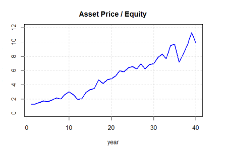As an illustrative example, consider the price and returns of a fictitious portfolio in the figure to the right. The x-axis represents yearly periods and the y- axis is the asset price. By inspection, we can see that that are years with positive and negative returns. (In this example, I generated the prices by sampling returns assuming 7% mean and 15% standard deviation).

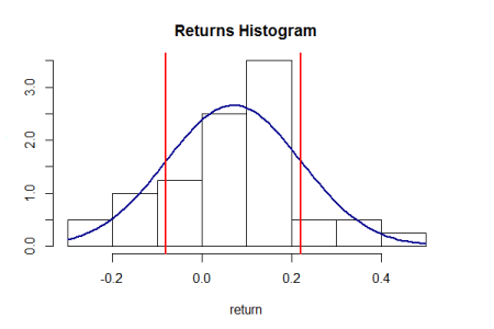In this next graph, I plotted a histogram of the actual returns for the asset above. First notice that the returns do seem to be centered around an average return of 7%. Next, notice that most of the returns fall within a range. For understanding, I added a red line at return levels of -8% and +22%. Finally, I added a blue curve that represents what we would expect to see if the returns follow a ‘normal’ or bell shaped curve.

Risk-Adjusted Return: Sharpe Ratio. When it comes to evaluating investments we always want to think in terms of both risk and return. One way convenient way to talk about risk-adjusted return is to use the Sharpe Ratio. The Sharpe Ratio expresses the return on an asset over the risk free rate, adjusted for risk. For simplicity, assume the risk free rate is 0%. Let’s take our 7% return and divide that by 15% standard deviation and we arrive at a Sharpe Ratio of .46. We would say that for each unit of risk, we will make .46% return. (Note. It is critical that the Sharpe Ratio be calculated using a common time period. For example, if our time period is one year, you would not want to use the monthly return / standard deviation as that will yield a far different result than for annual numbers).

If someone tells me that my money will generate X% return, the very next question we should ask is ‘how much risk will I be taking?’ Using measures like standard deviation we can express how much variation we can expect. Using the Sharpe Ratio we can normalize the return for assets with different levels of risk to get a better understanding of how assets with different risk compare to each other.

Long Term Measures for Risk, Return and Risk-Adjusted Return

Most investors have a time horizon of multiple years. Next let’s look at how we can talk about returns and risk when we are talking about multiple years of investing.

When it comes to returns, since the returns are variable, I like to talk about returns using a measure of the average return we might expect over the period. For risk, instead of looking at the typical variation for the returns, I like to look at the worst case scenario. How large of a drop in my portfolio could I expect? Examples of large drops in the market include the great depression and the financial crisis of 2007-2008.

Let’s look at the measures in more detail:

Return Measure: Compound Annual Rate of Return (CARG). I’d argue that this return measure is the most important measure for investors with a multiple year horizon. CAGR sounds complex but what it really does is give you the equivalent annual return you would need to explain the final return in your investment portfolio, given an initial investment. (For those interested in the formula and more discussion see: http://en.wikipedia.org/wiki/Compound_annual_growth_rate) .
An astute reader may say, ‘wait a minute, how will the CAGR be any different than the mean annual return?’ Answer: If there is no variation in the returns, then the CAGR will equal the mean annual return. Here is a key take-away. If the returns are variable, the effective return you will experience (called CAGR) will always be less than the mean return.

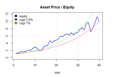As an example, let’s return to our fictitious asset price chart. I have added two curves to the chart. I have created the ‘green’ line to show the value of $1 invested at 7% return with no variation and compounded each year. We can see that our equity line for the asset falls below this curve. Why? Since the returns are variable, we have some good years and bad years. One way to think about why the variable return is low is to think about a drop of 25% in one year… Next year we may get a gain of 25% but that gain is not enough to make up for the 25% loss. We would need a larger gain to catch back up. When someone says ‘avoiding large losses’ is the key to investing, this curve example demonstrates the concept. If we can avoid large losses, we are more likely to achieve a higher average compounded return. In addition to the green line, I added the ‘red’ line to show what the value of $1 invested at 5.9% return with no variation. Notice that the starting value and ending value match our equity curve. The CAGR for the blue line is 5.9%. So another way to talk about CAGR is that it is the return with no variation that would result in the same ending value for our portfolio. When we are investing over the long term, certainly the ending value of the investment is a key goal and for this reason, CAGR helps us understand the multi-period return in a way that the mean return cannot.

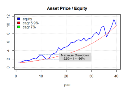Risk Measure: Maximum Drawdown. We could talk about the standard deviation for the annual returns, but for long horizons I also like to look at the maximum drawdown. Maximum drawdown is one of my favorite risk measures. It is intuitive to understand. It describes the maximum loss % from the peak value of an asset to its lowest value – it answers the questions, what is the most I could lose? Let’s return to our illustration. We can see periods where the asset price dropped below a previous high point. There are several periods or ‘drawdowns’ where this has occurred. In the illustration I highlight the large drawdown (measured on a percentage basis). At one point in the life of this investment, the asset price fell from 3 back down to 1.92. This represents a ‘drawdown’ of 36%. Note that visually the drop that occurs later is larger when measured in absolute value but the drop that occurs earlier in the cycle actually has a larger percentage fall.

Risk-Adjusted Return: Calmer Ratio. What about risk-adjusted return? For long periods of time I like to look at the CAGR divided by the Maximum Drawdown. This gives us an idea of the magnitude of the loss we could suffer against the expected long run average return. In this case, the Calmer Ratio = 5.9% / 36% = .44. For each % point maximum drop we are getting .44% return. Note that this ratio focuses on a worst-case scenario where the Sharpe Ratio gives us a measure of the typical risk-adjusted return. There is one word of caution I would add here. Large drops in the stock market are relatively infrequent. When we use ‘maximum drawdown’ and we derive that from history, then the result will be a function of how far we look back in history. Even with a long lookback the maximum drawdown may not be the worst case scenario.

Are there other practical reasons for looking at the Calmer Ratio vs. the Sharpe Ratio? I like to use Calmer for a number of reasons including the following:

• Calmer Ratio is useful when the variability in returns is not normal (i.e. where large drops are more likely than large gains – as is the case with stocks and alternative investments).
• Behavioral Factors. As humans we are prone to behavioral errors when we invest. For example, it is well known that during and after the 2007-2008 crash, investors pulled money from the market. Investors sell when the market is down and buy when it is peaking. Understanding and discussing the maximum drawdown gives us a way to proactively anticipate future investor concerns and manage investment behavioral biases.
• Retirement Planning. During retirement when the investor is drawing funds from their portfolio, large drops can have a particularly harsh effect on the retirement plan. Why? In effect, investors are forced to sell assets when they are down. The net effect of this is a drag on overall retirement success rate. For retirees, I am particularly concerned about the likelihood of large drawdowns are multiple years of bad returns. Avoiding large loses when we are in the distribution phase of a retirement plan is a key consideration.

Conclusion

Given that investments are not risk free, it is critical that we have a good grasp of how to measure, understand and discuss risk. Furthermore, we need to understand the difference between typical returns and worst case returns as well as the difference between average returns and effective returns in the face of variable returns. In this paper I have introduced return and risk measures that I think best help investors understand the risks they face. Once we have these tools we can more effectively evaluation portfolio performance, discuss future investment policies and make adjustments based on investor’s preferences and changing market conditions.